
Machine learning podział i informacje ogólne.
Klasyczne uczenie maszynowe
Supervised
Classification
- K-NN
- Naive Bayes
- SVM
- Decision Trees
- Logistic Regression
Regression
- Linear Regression
- Polynominal regression
- Ridge/Lasso regression
Unsupervised
Clustering
- DBSCAN
- K-Means (Flat)
- Agglomerative (Divisive: Bottom-up)
- Mean-Shift
- Fuzzy C-Means
📺 How does k-nearest neighbors work?
Pattern Search
- Euclat
- Apriori
- FP-Growth
Dimension Reduction
- t-SNE
- PCA
- LSA
- SVD
- LDA
Ensemble Methods
- Stacking
- Bagging
- Boosting
- AdaBoost
- XGBoost
- CatBoost
- LightGbm
Reinforcement Learning
- Genetic Algoritm
- Q-Learning
- Deep Q-Network (DQN)
- SARSA
- A3C
Sieci neuronowe
Perceptron (MLP)
Konwolucujne Sieci Neuronowe (CNN)
- DCNN
Recurrent Neutral Networks (RNN)
- LSM
- LSTM
- GRU
Autoencoders
- seq2seq
Generative Adversaliar Networks
https://renanmf.com/machine-learning-and-deep-learning-software-engineers/
- Korelacja
- Represents the relationship between two variables
- Shows that two variables move together (no matter in which direction)
- A single point (a number)
- Regresja
- Represents the relationship between two or more variables
- Shows cause and effect (one variable is affected by the other)
- One way – – there is always only one variable that is causally dependent
- A line (in 2D space)
Confusion matrix / ROC Curve
Underfitting - Overfiting
Overfiting - przeuczenie na danych treningowych. Zbyt małe uogólnienie modelu, za duże skoncentrowanie się na danych treningowych. High training accuracy. Lapie również wszystkie szumy
Underfiting - zbyt ogólny model, nie łapie o co chodzi nawet na treningowym. mało dokładny. Low train accuracy.
📺 Model Complexity Graph Detail Explanation
Loss function
Common Loss functions in machine learning
Sieci neuronowe (ANN)
Architektura najprostszej sieci neuronowej (MLP):
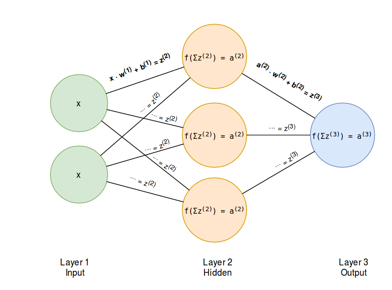
Źródło: Programming a neural network from scratch
Input layer - Dostarczają do sieci informacje ze świata zewnętrznego W żadnym z węzłów wejściowych nie są wykonywane żadne obliczenia - po prostu przekazują one informacje do ukrytych węzłów.
Hidden layer - Nie mają bezpośredniego połączenia ze światem zewnętrznym (stąd nazwa “ukryte”). Wykonują one obliczenia i przekazują informacje z węzłów wejściowych do węzłów wyjściowych. Kolekcja ukrytych węzłów tworzy “Ukrytą warstwę”. Sieć neuronowa ma tylko jedną warstwę wejściową i jedną warstwę wyjściową, może ona mieć zerową (Single Layer Perceptron) lub wielowarstwową (Multi Layer Perceptron) część ukrytą.
Output layer - Są odpowiedzialne za obliczenia i przesyłanie informacji z sieci do świata zewnętrznego.
Najczęstsze typy aktywacji
- Sigmoid (funkcja logistyczna). Zakres : (0,1)
- TanH (tangens hiperboliczny). Zakres (-1, 1)
- ReLu (rectified linear unit). Zakres (0, inf)
- SoftMax. Zakres: (0,1) Suma jest równa 1 (prawdopodobieństwo)
Przejście od warstwy wejściowej do wyjściowej to Feed Forward, Droga powrotna (OUT -> IN) to Back Propagation. Sieć uczy się i optymalizuje swój stan wewnętrzny poprzez minimalizowanie funkcji straty. Backdrop jest potrzebny żeby ustalić właściwe wagi i bias. Wykorzystuje gradienty, a żeby uniknąć pozostania w lokalnym minimum stosuje się Momentum.
Epoch is when an ENTIRE dataset is passed forward and backward through the neural network only ONCE
Batch - is a number of samples fed to NN during single iteration. Total number of training examples present in a single batch.
Iterations is the number of batches needed to complete one epoch.
Batch gradient descent computes the gradient using the whole dataset. This is great for convex, or relatively smooth error manifolds. In this case, we move somewhat directly towards an optimum solution, either local or global. Additionally, batch gradient descent, given an annealed learning rate, will eventually find the minimum located in it’s basin of attraction.
Stochastic gradient descent (SGD) computes the gradient using a single sample. Most applications of SGD actually use a minibatch of several samples, for reasons that will be explained a bit later. SGD works well (Not well, I suppose, but better than batch gradient descent) for error manifolds that have lots of local maxima/minima. In this case, the somewhat noisier gradient calculated using the reduced number of samples tends to jerk the model out of local minima into a region that hopefully is more optimal. Single samples are really noisy, while minibatches tend to average a little of the noise out. Thus, the amount of jerk is reduced when using minibatches. A good balance is struck when the minibatch size is small enough to avoid some of the poor local minima, but large enough that it doesn’t avoid the global minima or better-performing local minima. (Incidently, this assumes that the best minima have a larger and deeper basin of attraction, and are therefore easier to fall into.)
One benefit of SGD is that it’s computationally a whole lot faster. Large datasets often can’t be held in RAM, which makes vectorization much less efficient. Rather, each sample or batch of samples must be loaded, worked with, the results stored, and so on. Minibatch SGD, on the other hand, is usually intentionally made small enough to be computationally tractable.
Usually, this computational advantage is leveraged by performing many more iterations of SGD, making many more steps than conventional batch gradient descent. This usually results in a model that is very close to that which would be found via batch gradient descent, or better.
The way I like to think of how SGD works is to imagine that I have one point that represents my input distribution. My model is attempting to learn that input distribution. Surrounding the input distribution is a shaded area that represents the input distributions of all of the possible minibatches I could sample. It’s usually a fair assumption that the minibatch input distributions are close in proximity to the true input distribution. Batch gradient descent, at all steps, takes the steepest route to reach the true input distribution. SGD, on the other hand, chooses a random point within the shaded area, and takes the steepest route towards this point. At each iteration, though, it chooses a new point. The average of all of these steps will approximate the true input distribution, usually quite well.
Normalizacja
Więcej: Batch Normalization — Speed up Neural Network Training
-
Batch Gradient Descent (Batch Size == Number of samples)
-
Mini-Batch Gradient Descent ( 1 < Batch Size < Number of samples)
-
Stochasting Gradient Descent ( Batch Size ==1)
Regularyzacja
L1 - feature selection
L2 - zwykle lepsza do trenowania modeli
CNN
Warstwa konwolucyjna + pooling + ANN = CNN
# simple_cnn
Sequential([
 Conv2D(32, kernel_size=(3, 3), activation='relu', input_shape=input_shape),
 MaxPool2D(pool_size=(2, 2)),
 Dropout(0.25),

 Flatten(), # spłaszczanie, aby połączyć warstwy konwolucyjne z fully connected layers

 Dense(1024, activation='relu'),
 Dropout(0.5),
 Dense(num_classes, activation='softmax')
    ])
Konwolucja - nakładanie filtru (Image Kernels Explained Visually)
Pooling - sposób na zmniejszanie zdjęć przy jednoczesnym zachowaniu najważniejszych informacji w nich zawartych.
Capsule Networks - rozpoznawanie twarzy Blog post: capsule networks
Image augmentation - technika przeciwdziałania dla Rotate/scale/translation invariance (PyTorch: torchvision.transforms)